How processing (bundle adjustment) finds, or sometimes does not find, a solution

PhotoModeler’s main processing algorithm is called a bundle adjustment. ‘Bundle’ comes from the bundle of light rays from 3D points in the scene to images on the photos. ‘Adjustment’ comes the process of adjusting camera positions and 3D point positions given the defined bundle of light rays to minimize the overall error – that is, find the best 3D positions so the light ray bundle ‘makes sense’.

The algorithm is a type of search. We are searching for the best fit to the bundle of light rays. We are searching for the minimum or lowest error in the ‘fit’. A good visualization to help explain how it works is to use the analogy of a rectangular sheet made from thin rubber. A flat rubber sheet is a two dimensional (2D) surface. In this rubber sheet analogy we have a problem that has two values to solve (for example, the x value and the y value of a camera’s location in space). If we are solving two values, or parameters, we can say the distance along one edge of the sheet is parameter 1’s value, and the distance along the other edge is parameter 2’s value. Any single point on the sheet defines both values for the parameters.

Now press up on the rubber sheet from below to make mountains, ridges and valleys in the sheet. The height of the rubber is the ‘error’ – how far we are away from the solution. The higher the ‘mountain’, the higher the error and the worse the solution.

The deepest valley on the sheet is the best solution (closest to zero error) – that is, the best values for parameters 1 and 2. Find that deepest valley and you have the best solution and good values for x and y.

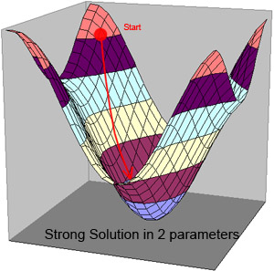
One way to find the deepest valley is to start with a ‘guess’ (or first approximation) for the two parameters – this is one point on the sheet – perhaps it lies on the side of a ‘mountain’. Now start walking downhill (towards smaller error). Or add a marble to the analogy and drop it somewhere on the sheet – let it roll downhill to find the lowest point. In the walking example, walk downhill until you are at the deepest valley point and you are at lowest error and you have the ‘solution’ – the best values for parameters 1 and 2. The solution is an iterative process. At each iteration, we look at where we are on the rubber sheet, look around us to find the steepest downward slope, and make a step in that direction. We repeat this at each iteration until we can’t find a direction that is ‘down’ from where we are currently. This usually means we are at the bottom of a hole or inverted cone. This may or may not be the lowest point on the whole rubber sheet.

The more vertically stretched the rubber sheet is (very tall mountains and one deep valley) the easier it is to start anywhere on the sheet and find the deepest valley (the correct solution). A sheet like this is a stable project that solves quickly. A strong project has one valley/hole that is deeper than all others and has steep sides.

A sheet that has many shallow holes/valleys and rounded/flat mountains will be harder to find the best and deepest valley.  A sheet like this is a weak project.  Depending on where you start on the sheet you may not find the lowest valley (you get caught in a false valley/sink-hole).

The weaker the project (which depends on the geometry of the camera stations and the points in the project) the flatter the sheet and the more false valleys (or multiple incorrect solutions) there are.

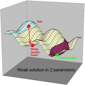
With a weak project you can still get to the right solution (lowest valley) if you start on the sheet near the correct valley – i.e. just up the hill from it.  If we get closer with the approximation to start, there is less chance bundle adjustment will get lost.

Strong projects (rubber sheets with high mountains and few deep valleys) solve easily and can solve even with poor first guess at the parameters. With weak projects (flatter rubber sheets and/or with multiple confusing valleys) you have to get closer with your first guess (orientation, constraint scaling) for it to solve. Often these weak projects will not solve (search gets lost) or will solve to the incorrect solution (cameras in the wrong place for example).

While the analogy above portrays just two parameters, the typical photogrammetric solution has hundreds or even thousands of parameters to solve.  Instead of a 2D rubber sheet we are in a multi-dimensional space – but the idea is still the same – walk ‘downhill’ towards lower error at each iteration to find the lowest error overall. Doing this efficiently, robustly and overcoming mathematical instabilities is where the advanced nature of the algorithms in PhotoModeler comes to play.

A strong photogrammetric project has strong angles between photos, a large number of 3d points, high precision marking, large coverage in each photo, and a good camera calibration.